
Dataset Viewer
pid
string | question
string | options
list | answer
string | image_1
image | image_2
image | image_3
image | image_4
image | image_5
image | solution
string | subject
string | task
string | category
string | source
string | type
string | context
string |
|---|---|---|---|---|---|---|---|---|---|---|---|---|---|---|---|
phy_30
|
A small toy car rolls down three ramps with the same height and horizontal length, but different shapes, starting from rest. The car stays in contact with the ramp at all times and no energy is lost. Order the ramps from the fastest to slowest time it takes for the toy car to drop the full $1 \mathrm{~m}$. For example, if ramp 1 is the fastest and ramp 3 is the slowest, then enter 123 as your answer choice.
Figure 1
<image_1>
Figure 2
<image_2>
Figure 3
<image_3>
|
[
"231",
"123",
"213",
"321"
] |
C
| Not supported with pagination yet | Not supported with pagination yet |
['One can solve this by finding the time it takes for each ramp. For ramp 1:\n$$\n\\begin{aligned}\n\\sqrt{2} & =\\frac{1}{2} g \\sin \\left(45^{\\circ}\\right) t^{2} \\\\\n\\Longrightarrow t & =0.639 \\mathrm{~s}\n\\end{aligned}\n$$\n\nFor ramps 2, let the length of the dashed region be $x$. Then:\n\n$$\nx+x / \\tan \\left(30^{\\circ}\\right)=1 \\Longrightarrow x=0.366 \\mathrm{~m}\n\\tag{1}\n$$\n\nDue to symmetry, both the steep and shallow regions of both ramps 2 and 3 have a length of $x / \\cos \\left(60^{\\circ}\\right)=0.732 \\mathrm{~m}$. This results in a time for ramp 2 as:\n\n$$\n\\begin{aligned}\n& 0.732=\\frac{1}{2} g \\sin \\left(60^{\\circ}\\right) t_{1}^{2} \\Longrightarrow t_{1}=0.415 \\mathrm{~s} \\\\\n& 0.732=\\sqrt{2 g(1-x)} t_{2}+\\frac{1}{2} g \\sin \\left(30^{\\circ}\\right) t_{2}^{2} \\Longrightarrow t_{2}=0.184 \\mathrm{~s}\n\\end{aligned}\n$$\n\nfor a total time of $t_{1}+t_{2}=0.599 \\mathrm{~s}$. For ramp 3 ,\n\n$$\n\\begin{aligned}\n& 0.732=\\frac{1}{2} g \\sin \\left(30^{\\circ}\\right) t_{1}^{2} \\Longrightarrow t_{1}=0.546 \\mathrm{~s} \\\\\n& 0.732=\\sqrt{2 g(1-x)} t_{2}+\\frac{1}{2} g \\sin \\left(60^{\\circ}\\right) t_{2}^{2} \\Longrightarrow t_{2}=0.206 \\mathrm{~s}\n\\end{aligned}\n$$\n\nwhich gives a total time of $t_{1}+t_{2}=0.752 \\mathrm{~s}$. From fastest to slowest, the answer becomes 213 . Note that this answer is easily guessable via intuition.']
|
Physics
|
Multi-hop Visual Reasoning
|
OlympiadBench
|
Multiple Choice
|
- Proton mass, $m_{p}=1.67 \cdot 10^{-27} \mathrm{~kg}$
- Neutron mass, $m_{n}=1.67 \cdot 10^{-27} \mathrm{~kg}$
- Electron mass, $m_{e}=9.11 \cdot 10^{-31} \mathrm{~kg}$
- Avogadro's constant, $N_{0}=6.02 \cdot 10^{23} \mathrm{~mol}^{-1}$
- Universal gas constant, $R=8.31 \mathrm{~J} /(\mathrm{mol} \cdot \mathrm{K})$
- Boltzmann's constant, $k_{B}=1.38 \cdot 10^{-23} \mathrm{~J} / \mathrm{K}$
- Electron charge magnitude, $e=1.60 \cdot 10^{-19} \mathrm{C}$
- 1 electron volt, $1 \mathrm{eV}=1.60 \cdot 10^{-19} \mathrm{~J}$
- Speed of light, $c=3.00 \cdot 10^{8} \mathrm{~m} / \mathrm{s}$
- Universal Gravitational constant,
$$
G=6.67 \cdot 10^{-11}\left(\mathrm{~N} \cdot \mathrm{m}^{2}\right) / \mathrm{kg}^{2}
$$
- Solar Mass
$$
M_{\odot}=1.988 \cdot 10^{30} \mathrm{~kg}
$$
- Acceleration due to gravity, $g=9.8 \mathrm{~m} / \mathrm{s}^{2}$
- 1 unified atomic mass unit,
$$
1 \mathrm{u}=1.66 \cdot 10^{-27} \mathrm{~kg}=931 \mathrm{MeV} / \mathrm{c}^{2}
$$
- Planck's constant,
$$
h=6.63 \cdot 10^{-34} \mathrm{~J} \cdot \mathrm{s}=4.41 \cdot 10^{-15} \mathrm{eV} \cdot \mathrm{s}
$$
- Permittivity of free space,
$$
\epsilon_{0}=8.85 \cdot 10^{-12} \mathrm{C}^{2} /\left(\mathrm{N} \cdot \mathrm{m}^{2}\right)
$$
- Coulomb's law constant,
$$
k=\frac{1}{4 \pi \epsilon_{0}}=8.99 \cdot 10^{9}\left(\mathrm{~N} \cdot \mathrm{m}^{2}\right) / \mathrm{C}^{2}
$$
- Permeability of free space,
$$
\mu_{0}=4 \pi \cdot 10^{-7} \mathrm{~T} \cdot \mathrm{m} / \mathrm{A}
$$
- Magnetic constant,
$$
\frac{\mu_{0}}{4 \pi}=1 \cdot 10^{-7}(\mathrm{~T} \cdot \mathrm{m}) / \mathrm{A}
$$
- 1 atmospheric pressure,
$$
1 \mathrm{~atm}=1.01 \cdot 10^{5} \mathrm{~N} / \mathrm{m}^{2}=1.01 \cdot 10^{5} \mathrm{~Pa}
$$
- Wien's displacement constant, $b=2.9$. $10^{-3} \mathrm{~m} \cdot \mathrm{K}$
- Stefan-Boltzmann constant,
$$
\sigma=5.67 \cdot 10^{-8} \mathrm{~W} / \mathrm{m}^{2} / \mathrm{K}^{4}
$$
|
||||
coding_524
|
<image_1>
<image_2>
Our goal is to reproduce the visualization in the first image shown. The code snippet below currently does not accurately generate the target visualization. It instead generates the visualization in the second image.
1 import matplotlib.pyplot as plt
2 import numpy as np
3 fig, ax = plt.subplots()
4 ax.set_xlim(0, 10)
5 ax.set_ylim(0, 10)
6 ax.set_xticks(np.arange(0, 11, 1))
7 ax.set_yticks(np.arange(0, 11, 1))
8 ax.grid(True, color="blue", linewidth=2)
9 main_diag = np.linspace(0, 10, 100)
10 ax.plot(main_diag, main_diag, color='lightgray', zorder=1)
11 ax.fill_betweenx(main_diag, main_diag - 1, main_diag + 1, color='lightblue', alpha=0.5, zorder=0)
12 solution_x = np.linspace(0, 10, 100)
13 solution_y = main_diag + 0.5 * np.sin(2 * np.pi * solution_x / 3)
14 ax.plot(solution_x, solution_y, color='red', linewidth=2, label='Solution')
15 ax.set_xlabel('Query', fontsize=12)
16 ax.set_ylabel('Reference', fontsize=12)
17 ax.text(5, 7, 'Main diagonal', fontsize=10, rotation=45, color='gray')
18 ax.text(7.5, 5, 'Solution Space', fontsize=10, rotation=0, color='black')
19 ax.text(8, 3, 'Solution', fontsize=10, rotation=0, color='red')
20 plt.show()
We are using Python version 3.11.0, matplotlib version 3.6.3, and seaborn version 0.12.2 (if applicable). What change should we apply to the original code in order to generate the target visualization?
|
[
"Replace lines 6-19 with:\nmain_diag = np.linspace(0, 10, 100)\nsolution_x = np.linspace(0, 10, 100)\nsolution_y = main_diag + 0.7 * np.sin(2 * np.pi * solution_x / 2.8)\nax.plot(solution_x, solution_y, color='red', linewidth=3, label='Solution')\nmajor_ticks = np.arange(0, 11, 2)\nax.set_xticks(major_ticks)\nax.set_yticks(major_ticks)\nax.tick_params(axis='both', which='both', length=0)\nax.vlines(major_ticks, ymin=0, ymax=10, colors='red', linewidth=1, zorder=0)\nax.hlines(major_ticks, xmin=0, xmax=10, colors='red', linewidth=1, zorder=0)\nminor_ticks = np.arange(2, 10, 1)\nax.vlines(minor_ticks, ymin=2, ymax=9, colors='blue', linewidth=1, zorder=0)\nax.hlines(minor_ticks, xmin=2, xmax=9, colors='blue', linewidth=1, zorder=0)\nmain_diag = np.linspace(0, 10, 100)\nax.plot(main_diag, main_diag, color='lightgray', linewidth=2, zorder=1)\nax.fill_betweenx(main_diag, main_diag - 2, main_diag + 2, color='lightblue', alpha=0.9, zorder=-1)\nax.set_xlabel('Query', fontsize=12)\nax.set_ylabel('Reference', fontsize=12)\nax.text(4, 6, 'Main diagonal', fontsize=10, rotation=45, color='gray')\nax.text(7, 3.5, 'Solution Space', fontsize=10, rotation=0, color='black')\nax.text(8.5, 1.5, 'Solution', fontsize=10, rotation=0, color='red')",
"Replace lines 6-19 with:\nax.set_xticks(np.arange(0, 11, 2))\nax.set_yticks(np.arange(0, 11, 2))\nax.grid(True, which='major', color='blue', linewidth=2)\nax.set_xticks(np.arange(2, 9, 1))\nax.set_yticks(np.arange(2, 9, 1))\nax.grid(True, which='minor', color='red', linewidth=2)\nmain_diag = np.linspace(0, 10, 100)\nax.plot(main_diag, main_diag, color='lightgray', linewidth=2, zorder=1)\nax.fill_betweenx(main_diag, main_diag - 2, main_diag + 2, color='lightblue', alpha=0.9, zorder=0)\nsolution_x = np.linspace(0, 10, 100)\nsolution_y = main_diag + 0.7 * np.sin(2 * np.pi * solution_x / 2.8)\nax.plot(solution_x, solution_y, color='red', linewidth=3, label='Solution')\nax.set_xlabel('Query', fontsize=12)\nax.set_ylabel('Reference', fontsize=12)\nax.text(4, 6, 'Main diagonal', fontsize=10, rotation=45, color='gray')\nax.text(7, 3.5, 'Solution Space', fontsize=10, rotation=0, color='black')\nax.text(8.5, 1.5, 'Solution', fontsize=10, rotation=0, color='red')",
"Replace lines 6-19 with:\nmain_diag = np.linspace(0, 10, 100)\nsolution_x = np.linspace(0, 10, 100)\nsolution_y = main_diag + 0.7 * np.sin(2 * np.pi * solution_x / 2.8)\nax.plot(solution_x, solution_y, color='red', linewidth=3, label='Solution')\nmajor_ticks = np.arange(0, 11, 2)\nax.set_xticks(major_ticks)\nax.set_yticks(major_ticks)\nax.tick_params(axis='both', which='both', length=0)\nax.vlines(major_ticks, ymin=0, ymax=10, colors='red', linewidth=2, zorder=0)\nax.hlines(major_ticks, xmin=0, xmax=10, colors='red', linewidth=2, zorder=0)\nminor_ticks = np.arange(2, 10, 1)\nax.vlines(minor_ticks, ymin=2, ymax=9, colors='blue', linewidth=2, zorder=0)\nax.hlines(minor_ticks, xmin=2, xmax=9, colors='blue', linewidth=2, zorder=0)\nmain_diag = np.linspace(0, 10, 100)\nax.plot(main_diag, main_diag, color='lightgray', linewidth=2, zorder=1)\nax.fill_betweenx(main_diag, main_diag - 2, main_diag + 2, color='lightblue', alpha=0.9, zorder=0)\nax.set_xlabel('Query', fontsize=12)\nax.set_ylabel('Reference', fontsize=12)\nax.text(4, 6, 'Main diagonal', fontsize=10, rotation=45, color='gray')\nax.text(7, 3.5, 'Solution Space', fontsize=10, rotation=0, color='black')\nax.text(8.5, 1.5, 'Solution', fontsize=10, rotation=0, color='red')",
"Replace lines 6-19 with:\nax.set_xticks(np.arange(0, 11, 2))\nax.set_yticks(np.arange(0, 11, 2))\nax.grid(True, which='major', color='red', linewidth=2)\nax.set_xticks(np.arange(2, 9, 1))\nax.set_yticks(np.arange(2, 9, 1))\nax.grid(True, which='minor', color='blue', linewidth=2)\nmain_diag = np.linspace(0, 10, 100)\nax.plot(main_diag, main_diag, color='lightgray', linewidth=2, zorder=1)\nax.fill_betweenx(main_diag, main_diag - 2, main_diag + 2, color='lightblue', alpha=0.9, zorder=0)\nsolution_x = np.linspace(0, 10, 100)\nsolution_y = main_diag + 0.7 * np.sin(2 * np.pi * solution_x / 2.8)\nax.plot(solution_x, solution_y, color='red', linewidth=3, label='Solution')\nax.set_xlabel('Query', fontsize=12)\nax.set_ylabel('Reference', fontsize=12)\nax.text(4, 6, 'Main diagonal', fontsize=10, rotation=45, color='gray')\nax.text(7, 3.5, 'Solution Space', fontsize=10, rotation=0, color='black')\nax.text(8.5, 1.5, 'Solution', fontsize=10, rotation=0, color='red')"
] |
D
| Not supported with pagination yet | Not supported with pagination yet | Not supported with pagination yet |
Coding
|
Modify With Image
|
Gridline;Color & Texture
|
new_annotated
|
Multiple Choice
| ||||
Math_301
|
A piece of string is lying on the table. It is partially covered by three coins as seen in the figure. Under each coin the string is equally likely to pass over itself like this: <image_1>
or like this: <image2>. What is the probability that the string is knotted after its ends are pulled?
|
[
"$\\frac{1}{2}$",
"$\\frac{1}{4}$",
"$\\frac{1}{8}$",
"$\\frac{3}{4}$",
"$\\frac{3}{8}$"
] |
B
| Not supported with pagination yet | Not supported with pagination yet | Not supported with pagination yet | Not supported with pagination yet | null |
Math
|
3D Spatial Simulation
|
MathVision
|
Multiple Choice
| |||
coding_319
|
<image_1>
Which code snippet below can possibly create the chart in the image? We are using Python version 3.11.0, matplotlib version 3.6.3, and seaborn version 0.12.2 (if applicable).
|
[
"import matplotlib.pyplot as plt\nfig, ax = plt.subplots(figsize=(6, 6))\ngrid_size = 8\nvoxel_mp1 = [(x, y) for x in range(grid_size) for y in range(grid_size)]\nvoxel_mp2 = [(2, 1), (3, 1), (2, 2), (3, 2), \n (5, 4), (6, 4), (5, 5), (6, 5), \n (1, 6), (2, 6), (1, 7), (2, 7)]\nfor x in range(grid_size):\n for y in range(grid_size):\n if (x, y) in voxel_mp2:\n ax.add_patch(plt.Rectangle((x, y), 1, 1, edgecolor='black', facecolor='brown'))\n else:\n ax.add_patch(plt.Rectangle((x, y), 1, 1, edgecolor='black', facecolor='lightblue'))\nfor x, y in voxel_mp1:\n ax.plot(x + 0.5, y + 0.5, 'o', color='gold', markersize=8)\nax.set_xlim(-1, grid_size)\nax.set_ylim(-1, grid_size)\nax.set_xticks([])\nax.set_yticks([])\nfor i in range(grid_size + 1):\n ax.plot([i - 0.5, i - 0.5], [-0.4, -0.6], color='goldenrod', lw=2)\n ax.plot([-0.4, -0.6], [i - 0.5, i - 0.5], color='goldenrod', lw=2)\nfor i in range(grid_size + 1):\n ax.text(i - 0.5, -0.85, str(i), ha='center', va='center', fontsize=12, color='goldenrod')\n ax.text(-0.85, i - 0.5, str(i), ha='center', va='center', fontsize=12, color='goldenrod')\nax.arrow(-0.5, -0.5, grid_size - 0.2, 0, head_width=0.3, head_length=0.3, fc='goldenrod', ec='goldenrod', lw=2)\nax.arrow(-0.5, -0.5, 0, grid_size - 0.2, head_width=0.3, head_length=0.3, fc='goldenrod', ec='goldenrod', lw=2)\nax.text(grid_size / 2, -1.25, 's1', ha='center', va='center', fontsize=14, color='goldenrod')\nax.text(-1.25, grid_size / 2, 's2', ha='center', va='center', fontsize=14, color='goldenrod', rotation=90)\nplt.text(-0.5, -1.75, 'Voxel (MP1)', color='lightblue', fontsize=12)\nplt.text(2, -1.75, 'Voxel (MP2)', color='brown', fontsize=12)\nplt.gca().set_aspect('equal', adjustable='box')\nplt.show()",
"import matplotlib.pyplot as plt\nfig, ax = plt.subplots(figsize=(6, 6))\ngrid_size = 8\nvoxel_mp1 = [(x, y) for x in range(grid_size) for y in range(grid_size)]\nvoxel_mp2 = [(2, 1), (3, 1), (2, 2), (3, 2), \n (5, 4), (6, 4), (5, 5), (6, 5), \n (1, 6), (2, 6), (1, 7), (2, 7)]\nfor x in range(grid_size):\n for y in range(grid_size):\n if (x, y) in voxel_mp2:\n ax.add_patch(plt.Rectangle((x, y), 1, 1, edgecolor='black', facecolor='brown'))\n else:\n ax.add_patch(plt.Rectangle((x, y), 1, 1, edgecolor='black', facecolor='lightblue'))\nfor x, y in voxel_mp1:\n ax.plot(x + 0.5, y + 0.5, 'o', color='gold', markersize=8)\nax.set_xlim(-1, grid_size)\nax.set_ylim(-1, grid_size)\nax.set_xticks([])\nax.set_yticks([])\nfor i in range(grid_size + 1):\n ax.plot([i - 0.5, i - 0.5], [-0.4, -0.6], color='goldenrod', lw=2)\n ax.plot([-0.4, -0.6], [i - 0.5, i - 0.5], color='goldenrod', lw=2)\n ax.plot([i - 0.5, i - 0.5], [grid_size + 0.4, grid_size + 0.6], color='goldenrod', lw=2)\n ax.plot([grid_size + 0.4, grid_size + 0.6], [i - 0.5, i - 0.5], color='goldenrod', lw=2)\nfor i in range(grid_size + 1):\n ax.text(i - 0.5, -0.85, str(i), ha='center', va='center', fontsize=12, color='goldenrod')\n ax.text(-0.85, i - 0.5, str(i), ha='center', va='center', fontsize=12, color='goldenrod')\n ax.text(i - 0.5, grid_size + 0.85, str(i), ha='center', va='center', fontsize=12, color='goldenrod')\n ax.text(grid_size + 0.85, i - 0.5, str(i), ha='center', va='center', fontsize=12, color='goldenrod')\nax.text(grid_size / 2, -1.25, 's1', ha='center', va='center', fontsize=14, color='goldenrod')\nax.text(-1.25, grid_size / 2, 's2', ha='center', va='center', fontsize=14, color='goldenrod', rotation=90)\nplt.text(-0.5, -1.75, 'Voxel (MP1)', color='lightblue', fontsize=12)\nplt.text(2, -1.75, 'Voxel (MP2)', color='brown', fontsize=12)\nplt.gca().set_aspect('equal', adjustable='box')\nplt.show()",
"import matplotlib.pyplot as plt\nfig, ax = plt.subplots(figsize=(6, 6))\ngrid_size = 8\nvoxel_mp1 = [(x, y) for x in range(grid_size) for y in range(grid_size)]\nvoxel_mp2 = [(2, 1), (3, 1), (2, 2), (3, 2), \n (5, 4), (6, 4), (5, 5), (6, 5), \n (1, 6), (2, 6), (1, 7), (2, 7)]\nfor x in range(grid_size):\n for y in range(grid_size):\n if (x, y) in voxel_mp2:\n ax.add_patch(plt.Rectangle((x, y), 1, 1, edgecolor='black', facecolor='brown'))\n else:\n ax.add_patch(plt.Rectangle((x, y), 1, 1, edgecolor='black', facecolor='lightblue'))\nfor x, y in voxel_mp1:\n ax.plot(x + 0.5, y + 0.5, 'o', color='gold', markersize=8)\nax.set_xlim(-1, grid_size)\nax.set_ylim(-1, grid_size)\nax.set_xticks([])\nax.set_yticks([])\nfor i in range(grid_size + 1):\n ax.plot([i - 0.5, i - 0.5], [0 - 0.1, 0 + 0.1], color='goldenrod', lw=2)\n ax.plot([-0.1, 0.1], [i - 0.5, i - 0.5], color='goldenrod', lw=2)\nfor i in range(grid_size + 1):\n ax.text(i - 0.5, -0.25, str(i), ha='center', va='center', fontsize=12, color='goldenrod')\n ax.text(-0.25, i - 0.5, str(i), ha='center', va='center', fontsize=12, color='goldenrod')\nax.arrow(-0.5, -0.5, grid_size - 0.2, 0, head_width=0.3, head_length=0.3, fc='goldenrod', ec='goldenrod', lw=2)\nax.arrow(-0.5, -0.5, 0, grid_size - 0.2, head_width=0.3, head_length=0.3, fc='goldenrod', ec='goldenrod', lw=2)\nax.text(grid_size / 2, -1.25, 's1', ha='center', va='center', fontsize=14, color='goldenrod')\nax.text(-1.25, grid_size / 2, 's2', ha='center', va='center', fontsize=14, color='goldenrod', rotation=90)\nplt.text(-0.5, -1.75, 'Voxel (MP1)', color='lightblue', fontsize=12)\nplt.text(2, -1.75, 'Voxel (MP2)', color='brown', fontsize=12)\nplt.gca().set_aspect('equal', adjustable='box')\nplt.show()",
"import matplotlib.pyplot as plt\nfig, ax = plt.subplots(figsize=(6, 6))\ngrid_size = 8\nvoxel_mp1 = [(x, y) for x in range(grid_size) for y in range(grid_size)]\nvoxel_mp2 = [(2, 1), (3, 1), (2, 2), (3, 2), \n (5, 4), (6, 4), (5, 5), (6, 5), \n (1, 6), (2, 6), (1, 7), (2, 7)]\nfor x in range(grid_size):\n for y in range(grid_size):\n if (x, y) in voxel_mp2:\n ax.add_patch(plt.Rectangle((x, y), 1, 1, edgecolor='black', facecolor='brown'))\n else:\n ax.add_patch(plt.Rectangle((x, y), 1, 1, edgecolor='black', facecolor='lightblue'))\nfor x, y in voxel_mp1:\n ax.plot(x + 0.5, y + 0.5, 'o', color='gold', markersize=8)\nax.set_xlim(-1, grid_size)\nax.set_ylim(-1, grid_size)\nax.set_xticks([])\nax.set_yticks([])\nfor i in range(grid_size + 1):\n ax.plot([i - 0.5, i - 0.5], [-0.4, -0.6], color='goldenrod', lw=2)\n ax.plot([-0.4, -0.6], [i - 0.5, i - 0.5], color='goldenrod', lw=2)\nfor i in range(grid_size + 1):\n ax.text(i - 0.5, -0.85, str(i), ha='center', va='center', fontsize=12, color='goldenrod')\n ax.text(-0.85, i - 0.5, str(i), ha='center', va='center', fontsize=12, color='goldenrod')\nax.plot([0, grid_size - 0.5], [-0.5, -0.5], color='goldenrod', lw=2) \nax.plot([-0.5, -0.5], [0, grid_size - 0.5], color='goldenrod', lw=2) \nax.text(grid_size / 2, -1.25, 's1', ha='center', va='center', fontsize=14, color='goldenrod')\nax.text(-1.25, grid_size / 2, 's2', ha='center', va='center', fontsize=14, color='goldenrod', rotation=90)\nplt.text(-0.5, -1.75, 'Voxel (MP1)', color='lightblue', fontsize=12)\nplt.text(2, -1.75, 'Voxel (MP2)', color='brown', fontsize=12)\nplt.gca().set_aspect('equal', adjustable='box')\nplt.show()"
] |
C
| Not supported with pagination yet | Not supported with pagination yet | Not supported with pagination yet | Not supported with pagination yet |
Coding
|
Vis Choose Code
|
Advanced Chart Type;Axis & Scale
|
new_annotated
|
Multiple Choice
| |||
chem_82
|
<image_1> An 'arrow-pushing' diagram is a common type of chemical image used to illustrate electron flow in mechanistic steps. The transition-state structure undergoes changes after the electron has been relocated or reacted. Which of the following options shows the structure after the change? Note: Disregard the arrows in the options. The selected option should represent the immediate product of the next step, not the final product of the reaction.
|
[
"<image_2>",
"<image_3>",
"<image_4>",
"<image_5>"
] |
D
|
Chemistry
|
Reaction Simulation Pro
|
new_annotated
|
Multiple choice
| ||||||||
chem_324
|
<image_1> In the transition-state structure shown in the image, calculate the total number of bonds in the structure, including single, double, and triple bonds but excluding those involving hydrogen.
Note: Disregard arrows. Consider all components present in the transition-state structure shown in the image.
|
[] |
4
| Not supported with pagination yet | Not supported with pagination yet | Not supported with pagination yet | Not supported with pagination yet |
Chemistry
|
Knowledge-based counting
|
new_annotated
|
Open-ended
| ||||
phy_95
|
A disk of radius $a/4$ having a uniformly distributed charge $6C$ is placed in the $x$-y plane with its centre at $(-a/2, 0, 0)$. A rod of length $a$ carrying a uniformly distributed charge $8C$ is placed on the $x$-axis from $x = a/4$ to $x = 5a/4$. Two point charges $-7C$ and $3C$ are placed at $(a/4, -a/4, 0)$ and $(-3a/4, 3a/4, 0)$, respectively. Consider a cubical surface formed by six surfaces $x = \pm a/2$, $y = \pm a/2$, $z = \pm a/2$. The electric flux through this cubical surface is
<image_1>
|
[
"$\\frac{-2C}{\\varepsilon_0}$",
"$\\frac{2C}{\\varepsilon_0}$",
"$\\frac{10C}{\\varepsilon_0}$",
"$\\frac{12C}{\\varepsilon_0}$"
] |
A
| Not supported with pagination yet | Not supported with pagination yet | Not supported with pagination yet | Not supported with pagination yet |
Physics
|
3d Field Simulation
|
EXAMS-V
|
Multiple Choice
| ||||
Math_334
|
The big cube is made up of three different kinds of building blocks (see diagram). How many of the little white cubes are needed for this big cube?
<image_1>
|
[] |
11
| Not supported with pagination yet | Not supported with pagination yet | Not supported with pagination yet | Not supported with pagination yet | null |
Math
|
3D Spatial Simulation
|
MathVision
|
Open-ended
| |||
chem_1120
|
An 'arrow-pushing' diagram is a common type of chemical image used to illustrate electron flow in mechanistic steps. Please choose the SMILES expression for the molecules(state) after the electron has been relocated, as depicted in the image. <image_1>
|
[
"Br[C-](Br)Br.Br[P+](c1ccccc1)(c2ccccc2)(c3ccccc3)",
"Br[C-](Br)(Br)Br.Br[P+](c1ccccc1)(c2ccccc2)c3ccccc3",
"Br[C-](Br)Br.Br[P+](c1ccccc1)(c2ccccc2)c4ccccc4",
"Br[C-](Br)Br.Br[P+](c1ccccc1)(c2ccccc2)c3ccccc3"
] |
D
| Not supported with pagination yet | Not supported with pagination yet | Not supported with pagination yet | Not supported with pagination yet |
Chemistry
|
Reaction Simulation
|
new_annotated
|
Multiple choice
| ||||
chem_108
|
P is the probability of finding the 1s electron of hydrogen atom in a spherical shell of infinitesimal thickness, dr, at a distance r from the nucleus. The volume of this shell is 4$\pi r^2$dr. The qualitative sketch of the dependence of P on r is <image_1>
|
[
"A",
"B",
"C",
"D"
] |
D
| Not supported with pagination yet | Not supported with pagination yet | Not supported with pagination yet | Not supported with pagination yet |
Chemistry
|
Graph Reasoning
|
EXAMS-V
|
Multiple choice
| ||||
Math_711
|
<image_1>
Is the number of metal cars that are left of the tiny matte school bus greater than the number of tiny cyan double buss?
|
[
"Yes",
"No"
] |
A
| Not supported with pagination yet | Not supported with pagination yet | Not supported with pagination yet | Not supported with pagination yet |
Math
|
Multi-hop Visual Object Counting
|
MathVista
|
Multiple Choice
| ||||
coding_486
|
<image_1>
<image_2>
Our goal is to reproduce the visualization in the first image shown. The code snippet below currently does not accurately generate the target visualization. It instead generates the visualization in the second image.
1 import matplotlib.pyplot as plt
2 import numpy as np
3 import seaborn as sns
4 import pandas as pd
5 np.random.seed(0)
6 sns.set(style="whitegrid")
7 x1 = np.random.normal(0.85, 0.1, 100)
8 y1 = x1 + np.random.normal(0, 0.1, 100)
9 x2 = np.random.normal(0.9, 0.1, 100)
10 y2 = x2 + np.random.normal(0, 0.1, 100)
11 data1 = pd.DataFrame({'Std dose of CDDP+DOX (Delta)': x1, 'RDI': y1, 'HRe': np.random.choice(['Poor', 'Good'], 100)})
12 data2 = pd.DataFrame({'Std dose of CDDP+DOX (Delta)': x2, 'RDI': y2, 'HRe': np.random.choice(['Poor', 'Good'], 100)})
13 fig, axes = plt.subplots(1, 2, figsize=(12, 5), sharey=True)
14 sns.scatterplot(ax=axes[0], data=data1, x='Std dose of CDDP+DOX (Delta)', y='RDI', hue='HRe', palette={'Poor': 'blue', 'Good': 'green'}, s=50)
15 axes[0].plot([0.4, 1.2], [0.4, 1.2], color='black')
16 axes[0].axhline(0.85, color='red', linestyle='--')
17 axes[0].axhline(0.55, color='red', linestyle='--')
18 axes[0].set_title('BO03 trial')
19 sns.scatterplot(ax=axes[1], data=data2, x='Std dose of CDDP+DOX (Delta)', y='RDI', hue='HRe', palette={'Poor': 'blue', 'Good': 'green'}, s=50)
20 axes[1].plot([0.4, 1.2], [0.4, 1.2], color='black')
21 axes[1].axhline(0.85, color='red', linestyle='--')
22 axes[1].axhline(0.55, color='red', linestyle='--')
23 axes[1].set_title('BO06 trial')
24 plt.tight_layout()
25 plt.show()
We are using Python version 3.11.0, matplotlib version 3.6.3, and seaborn version 0.12.2 (if applicable). What change should we apply to the original code in order to generate the target visualization?
|
[
"Replace line 6 with:\nsns.set(style=\"ggplot2\")",
"Replace lines 6-23 with:\nsns.set(style=\"dark\")\nx1 = np.random.normal(0.85, 0.1, 100)\ny1 = x1 + np.random.normal(0, 0.1, 100)\nx2 = np.random.normal(0.9, 0.1, 100)\ny2 = x2 + np.random.normal(0, 0.1, 100)\ndata1 = pd.DataFrame({'Std dose of CDDP+DOX (Delta)': x1, 'RDI': y1, 'HRe': np.random.choice(['Poor', 'Good'], 100)})\ndata2 = pd.DataFrame({'Std dose of CDDP+DOX (Delta)': x2, 'RDI': y2, 'HRe': np.random.choice(['Poor', 'Good'], 100)})\nfig, axes = plt.subplots(1, 2, figsize=(12, 5), sharey=True)\nsns.scatterplot(ax=axes[0], data=data1, x='Std dose of CDDP+DOX (Delta)', y='RDI', hue='HRe', palette={'Poor': 'blue', 'Good': 'green'}, s=50)\naxes[0].plot([0.4, 1.2], [0.4, 1.2], color='black')\naxes[0].axhline(0.85, color='red', linestyle='--')\naxes[0].axhline(0.55, color='red', linestyle='--')\naxes[0].set_title('BO03 trial')\naxes[0].grid(True)\nsns.scatterplot(ax=axes[1], data=data2, x='Std dose of CDDP+DOX (Delta)', y='RDI', hue='HRe', palette={'Poor': 'blue', 'Good': 'green'}, s=50)\naxes[1].plot([0.4, 1.2], [0.4, 1.2], color='black')\naxes[1].axhline(0.85, color='red', linestyle='--')\naxes[1].axhline(0.55, color='red', linestyle='--')\naxes[1].set_title('BO06 trial')\naxes[1].grid(True)",
"Replace lines 6-19 with:\nx1 = np.random.normal(0.85, 0.1, 100)\ny1 = x1 + np.random.normal(0, 0.1, 100)\nx2 = np.random.normal(0.9, 0.1, 100)\ny2 = x2 + np.random.normal(0, 0.1, 100)\ndata1 = pd.DataFrame({'Std dose of CDDP+DOX (Delta)': x1, 'RDI': y1, 'HRe': np.random.choice(['Poor', 'Good'], 100)})\ndata2 = pd.DataFrame({'Std dose of CDDP+DOX (Delta)': x2, 'RDI': y2, 'HRe': np.random.choice(['Poor', 'Good'], 100)})\nfig, axes = plt.subplots(1, 2, figsize=(12, 5), sharey=True)\nsns.scatterplot(ax=axes[0], data=data1, x='Std dose of CDDP+DOX (Delta)', y='RDI', hue='HRe', palette={'Poor': 'blue', 'Good': 'green'})\naxes[0].plot([0.4, 1.2], [0.4, 1.2], color='black')\naxes[0].axhline(0.85, color='red', linestyle='--')\naxes[0].axhline(0.55, color='red', linestyle='--')\naxes[0].set_title('BO03 trial')\nsns.scatterplot(ax=axes[1], data=data2, x='Std dose of CDDP+DOX (Delta)', y='RDI', hue='HRe', palette={'Poor': 'blue', 'Good': 'green'})",
"Replace lines 6-23 with:\nsns.set(style=\"classic\")\nx1 = np.random.normal(0.85, 0.1, 100)\ny1 = x1 + np.random.normal(0, 0.1, 100)\nx2 = np.random.normal(0.9, 0.1, 100)\ny2 = x2 + np.random.normal(0, 0.1, 100)\ndata1 = pd.DataFrame({'Std dose of CDDP+DOX (Delta)': x1, 'RDI': y1, 'HRe': np.random.choice(['Poor', 'Good'], 100)})\ndata2 = pd.DataFrame({'Std dose of CDDP+DOX (Delta)': x2, 'RDI': y2, 'HRe': np.random.choice(['Poor', 'Good'], 100)})\nfig, axes = plt.subplots(1, 2, figsize=(12, 5), sharey=True)\nsns.scatterplot(ax=axes[0], data=data1, x='Std dose of CDDP+DOX (Delta)', y='RDI', hue='HRe', palette={'Poor': 'blue', 'Good': 'green'}, s=50)\naxes[0].plot([0.4, 1.2], [0.4, 1.2], color='black')\naxes[0].axhline(0.85, color='red', linestyle='--')\naxes[0].axhline(0.55, color='red', linestyle='--')\naxes[0].set_title('BO03 trial')\naxes[0].grid(True)\nsns.scatterplot(ax=axes[1], data=data2, x='Std dose of CDDP+DOX (Delta)', y='RDI', hue='HRe', palette={'Poor': 'blue', 'Good': 'green'}, s=50)\naxes[1].plot([0.4, 1.2], [0.4, 1.2], color='black')\naxes[1].axhline(0.85, color='red', linestyle='--')\naxes[1].axhline(0.55, color='red', linestyle='--')\naxes[1].set_title('BO06 trial')\naxes[1].grid(True)"
] |
C
| Not supported with pagination yet | Not supported with pagination yet | Not supported with pagination yet |
Coding
|
Modify With Image
|
Gridline
|
new_annotated
|
Multiple Choice
| ||||
Math_441
|
A cube is being rolled on a plane so it turns around its edges. Its bottom face passes through the positions $1,2,3,4,5,6$ and 7 in that order, as shown. Which of these two positions were occupied by the same face of the cube? <image_1>
|
[
"1 and 7",
"1 and 6",
"1 and 5",
"2 and 7",
"2 and 6"
] |
B
| Not supported with pagination yet | Not supported with pagination yet | Not supported with pagination yet | Not supported with pagination yet |
Imagine the grid is sticky so that when the cube rolls over it, each cell of the grid fastens to the face of the cube touching it. The result would be equivalent to taking the arrangement of cells as shown, cutting it out and folding it into a cube. The latter is possible (for example) with 5 on 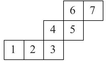 the bottom, 6 at the back, 7 on the right, 4 on the left, 3 at the front, 2 on the top and 1 folding over the 6 at the back. Hence 1 and 6 are occupied by the same face of the cube.
|
Math
|
3D Spatial Simulation
|
MathVision
|
Multiple Choice
| |||
chem_244
|
<image_1> In the transition-state structure shown in the image, calculate the total number of bonds in the structure, including single, double, and triple bonds but excluding those involving hydrogen.
Note: Disregard arrows. Consider all components present in the transition-state structure shown in the image.
|
[] |
15
| Not supported with pagination yet | Not supported with pagination yet | Not supported with pagination yet | Not supported with pagination yet |
Chemistry
|
Knowledge-based counting
|
new_annotated
|
Open-ended
| ||||
chem_368
|
<image_1> In the transition-state structure shown in the image, calculate the total number of bonds in the structure, including single, double, and triple bonds but excluding those involving hydrogen.
Note: Disregard arrows. Consider all components present in the transition-state structure shown in the image.
|
[] |
18
| Not supported with pagination yet | Not supported with pagination yet | Not supported with pagination yet | Not supported with pagination yet |
Chemistry
|
Knowledge-based counting
|
new_annotated
|
Open-ended
| ||||
Math_291
|
The diagram shows an object made up of 12 dice glued-together. The object is dipped into some colour so that the entire outside is coloured in this new colour. How many of the small dice will have exactly four faces coloured in?
<image_1>
|
[] |
10
| Not supported with pagination yet | Not supported with pagination yet | Not supported with pagination yet | Not supported with pagination yet | null |
Math
|
3D Spatial Simulation
|
MathVision
|
Open-ended
| |||
chem_592
|
<image_1> In the transition-state structure shown in the image, calculate the total number of bonds in the structure, including single, double, and triple bonds but excluding those involving hydrogen.
Note: Disregard arrows. Consider all components present in the transition-state structure shown in the image.
|
[] |
10
| Not supported with pagination yet | Not supported with pagination yet | Not supported with pagination yet | Not supported with pagination yet |
Chemistry
|
Knowledge-based counting
|
new_annotated
|
Open-ended
| ||||
coding_538
|
<image_1>
<image_2>
Our goal is to reproduce the visualization in the first image shown. The code snippet below currently does not accurately generate the target visualization. It instead generates the visualization in the second image.
1 import matplotlib.pyplot as plt
2 import numpy as np
3 np.random.seed(0)
4 from matplotlib.patches import Patch
5 data = [np.random.normal(0, 1, 10000) for _ in range(4)]
6 hatches = ['/', 'X', '|', '\\']
7 labels = [f'set {i}' for i in range(1, 5)]
8 bins = 30
9 hist_data = [np.histogram(d, bins=bins)[0] for d in data]
10 bin_edges = np.histogram(data[0], bins=bins)[1]
11 bin_width = bin_edges[1] - bin_edges[0]
12 bin_centers = bin_edges[:-1] + bin_width / 2
13 bottom = np.zeros(bins)
14 fig, ax = plt.subplots(figsize=(10, 7))
15 for i in range(4):
16 ax.bar(
17 bin_centers,
18 hist_data[i],
19 width=bin_width,
20 bottom=bottom,
21 edgecolor='black',
22 label=labels[i],
23 hatch=hatches[i],
24 alpha=0.7
25 )
26 bottom += hist_data[i]
27 ax.set_xlabel('x')
28 ax.set_ylabel('Counts')
29 colors = ['tab:blue', 'tab:orange', 'tab:green', 'tab:red']
30 legend_patches = [Patch(facecolor=colors[i], edgecolor='black', hatch=hatches[i], label=labels[i], alpha=0.7) for i in range(4)]
31 ax.legend(handles=legend_patches, title="Datasets")
32 plt.show()
We are using Python version 3.11.0, matplotlib version 3.6.3, and seaborn version 0.12.2 (if applicable). What change should we apply to the original code in order to generate the target visualization?
|
[
"Replace lines 4-31 with:\ndata = [np.random.normal(0, 1, 10000) for _ in range(4)]\nfig, ax = plt.subplots()\nhatches = ['/', '*', '|', '']\nlabels = [f'set {i}' for i in range(4)]\nfor i in range(4):\n ax.hist(data[i], bins=30, alpha=0.5, label=labels[i],\n edgecolor='black', hatch=hatches[i], histtype='barstacked')\nax.set_xlabel('x')\nax.set_ylabel('counts')\nax.legend()",
"Replace line 6 with:\nhatches = ['/', '*', '|', '\\\\']",
"Replace lines 4-31 with:\ndata = [np.random.normal(0, 1, 10000) for _ in range(4)]\nfig, ax = plt.subplots()\nhatches = ['/', 'X', '|', '']\nlabels = [f'set {i}' for i in range(4)]\nfor i in range(4):\n ax.hist(data[i], bins=30, alpha=0.5, label=labels[i],\n edgecolor='black', hatch=hatches[i], histtype='barstacked')\nax.set_xlabel('x')\nax.set_ylabel('counts')\nax.legend()",
"Replace line 6 with:\nhatches = ['o', 'X', '.', '\\\\']"
] |
C
| Not supported with pagination yet | Not supported with pagination yet | Not supported with pagination yet |
Coding
|
Modify With Image
|
Color & Texture;Advanced Chart Type;Alignment, Orientation, & Position
|
new_annotated
|
Multiple Choice
| ||||
phy_83
|
The x-t graph of a particle undergoing simple harmonic motion is shown below. The acceleration of the particle at t = 4/3 s is
<image_1>
|
[
"$\\frac{\\sqrt{3}}{32}\\pi^2$ cm/s$^2$",
"$\\frac{-\\pi^2}{32}$ cm/s$^2$",
"$\\frac{\\pi^2}{32}$ cm/s$^2$",
"$-\\frac{\\sqrt{3}}{32}\\pi^2$ cm/s$^2$"
] |
D
| Not supported with pagination yet | Not supported with pagination yet | Not supported with pagination yet | Not supported with pagination yet |
Physics
|
Graph Reasoning
|
EXAMS-V
|
Multiple Choice
| ||||
coding_523
|
<image_1>
<image_2>
Our goal is to reproduce the visualization in the first image shown. The code snippet below currently does not accurately generate the target visualization. It instead generates the visualization in the second image.
1 import matplotlib.pyplot as plt
2 import numpy as np
3 fig, ax = plt.subplots()
4 ax.set_xlim(0, 10)
5 ax.set_ylim(0, 10)
6 ax.set_xticks(np.arange(0, 11, 2))
7 ax.set_yticks(np.arange(0, 11, 2))
8 ax.grid(True, which='major', color='red', linewidth=2)
9 ax.set_xticks(np.arange(2, 9, 1))
10 ax.set_yticks(np.arange(2, 9, 1))
11 ax.grid(True, which='minor', color='blue', linewidth=2)
12 main_diag = np.linspace(0, 10, 100)
13 ax.plot(main_diag, main_diag, color='lightgray', linewidth=2, zorder=1)
14 ax.fill_betweenx(main_diag, main_diag - 2, main_diag + 2, color='lightblue', alpha=0.9, zorder=0)
15 solution_x = np.linspace(0, 10, 100)
16 solution_y = main_diag + 0.7 * np.sin(2 * np.pi * solution_x / 2.8)
17 ax.plot(solution_x, solution_y, color='red', linewidth=3, label='Solution')
18 ax.set_xlabel('Query', fontsize=12)
19 ax.set_ylabel('Reference', fontsize=12)
20 ax.text(4, 6, 'Main diagonal', fontsize=10, rotation=45, color='gray')
21 ax.text(7, 3.5, 'Solution Space', fontsize=10, rotation=0, color='black')
22 ax.text(8.5, 1.5, 'Solution', fontsize=10, rotation=0, color='red')
23 plt.show()
We are using Python version 3.11.0, matplotlib version 3.6.3, and seaborn version 0.12.2 (if applicable). What change should we apply to the original code in order to generate the target visualization?
|
[
"Replace lines 8-11 with:\nax.grid(True, which='major', color='blue', linewidth=2)\nax.set_xticks(np.arange(2, 9, 1))\nax.set_yticks(np.arange(2, 9, 1))\nax.grid(True, which='minor', color='red', linewidth=2)",
"Replace lines 6-17 with:\nmain_diag = np.linspace(0, 10, 100)\nsolution_x = np.linspace(0, 10, 100)\nsolution_y = main_diag + 0.7 * np.sin(2 * np.pi * solution_x / 2.8)\nax.plot(solution_x, solution_y, color='red', linewidth=3, label='Solution')\nmajor_ticks = np.arange(0, 11, 2)\nax.set_xticks(major_ticks)\nax.set_yticks(major_ticks)\nax.tick_params(axis='both', which='both', length=0)\nax.vlines(major_ticks, ymin=0, ymax=10, colors='red', linewidth=2, zorder=0)\nax.hlines(major_ticks, xmin=0, xmax=10, colors='red', linewidth=2, zorder=0)\nminor_ticks = np.arange(2, 10, 1)\nax.vlines(minor_ticks, ymin=2, ymax=9, colors='blue', linewidth=2, zorder=0)\nax.hlines(minor_ticks, xmin=2, xmax=9, colors='blue', linewidth=2, zorder=0)\nmain_diag = np.linspace(0, 10, 100)\nax.plot(main_diag, main_diag, color='lightgray', linewidth=2, zorder=1)\nax.fill_betweenx(main_diag, main_diag - 2, main_diag + 2, color='lightblue', alpha=0.9, zorder=0)",
"Replace lines 6-22 with:\nax.set_xticks(np.arange(0, 11, 1))\nax.set_yticks(np.arange(0, 11, 1))\nax.grid(True, color=\"blue\", linewidth=2)\nmain_diag = np.linspace(0, 10, 100)\nax.plot(main_diag, main_diag, color='lightgray', zorder=1)\nax.fill_betweenx(main_diag, main_diag - 1, main_diag + 1, color='lightblue', alpha=0.5, zorder=0)\nsolution_x = np.linspace(0, 10, 100)\nsolution_y = main_diag + 0.5 * np.sin(2 * np.pi * solution_x / 3)\nax.plot(solution_x, solution_y, color='red', linewidth=2, label='Solution')\nax.set_xlabel('Query', fontsize=12)\nax.set_ylabel('Reference', fontsize=12)\nax.text(5, 7, 'Main diagonal', fontsize=10, rotation=45, color='gray')\nax.text(7.5, 5, 'Solution Space', fontsize=10, rotation=0, color='black')\nax.text(8, 3, 'Solution', fontsize=10, rotation=0, color='red')",
"Replace lines 6-17 with:\nmain_diag = np.linspace(0, 10, 100)\nsolution_x = np.linspace(0, 10, 100)\nsolution_y = main_diag + 0.7 * np.sin(2 * np.pi * solution_x / 2.8)\nax.plot(solution_x, solution_y, color='red', linewidth=3, label='Solution')\nmajor_ticks = np.arange(0, 11, 2)\nax.set_xticks(major_ticks)\nax.set_yticks(major_ticks)\nax.tick_params(axis='both', which='both', length=0)\nax.vlines(major_ticks, ymin=0, ymax=10, colors='red', linewidth=1, zorder=0)\nax.hlines(major_ticks, xmin=0, xmax=10, colors='red', linewidth=1, zorder=0)\nminor_ticks = np.arange(2, 10, 1)\nax.vlines(minor_ticks, ymin=2, ymax=9, colors='blue', linewidth=1, zorder=0)\nax.hlines(minor_ticks, xmin=2, xmax=9, colors='blue', linewidth=1, zorder=0)\nmain_diag = np.linspace(0, 10, 100)\nax.plot(main_diag, main_diag, color='lightgray', linewidth=2, zorder=1)\nax.fill_betweenx(main_diag, main_diag - 2, main_diag + 2, color='lightblue', alpha=0.9, zorder=-1)"
] |
B
| Not supported with pagination yet | Not supported with pagination yet | Not supported with pagination yet |
Coding
|
Modify With Image
|
Gridline;Color & Texture
|
new_annotated
|
Multiple Choice
| ||||
Math_722
|
<image_1>
Are there fewer jets that are left of the small brown suv than objects right of the big shiny car?
|
[
"Yes",
"No"
] |
A
| Not supported with pagination yet | Not supported with pagination yet | Not supported with pagination yet | Not supported with pagination yet |
Math
|
Multi-hop Visual Object Counting
|
MathVista
|
Multiple Choice
| ||||
phy_77
|
A parallel plate capacitor $C$ with plates of unit area and separation $d$ is filled with a liquid of dielectric constant $K=2$. The level of liquid is $\frac{d}{3}$ initially. Suppose the liquid level decreases at a constant speed $V$, the time constant as a function of time $t$ is
<image_1>
|
[
"$\\frac{6\\epsilon_0R}{5d+3Vt}$",
"$\\frac{(15d+9Vt)\\epsilon_0R}{2d^2-3dVt-9V^2t^2}$",
"$\\frac{6\\epsilon_0R}{5d-3Vt}$",
"$\\frac{(15d-9Vt)\\epsilon_0R}{2d^2+3dVt-9V^2t^2}$"
] |
A
| Not supported with pagination yet | Not supported with pagination yet | Not supported with pagination yet | Not supported with pagination yet |
Physics
|
Multi-hop Visual Reasoning
|
EXAMS-V
|
Multiple Choice
| ||||
Math_40
|
At noon the minute hand of a clock is in the position shown on the left and after the quarter of an hour -- in the position shown on the right. Which position the minute hand will take after seventeen quarters from the noon?
<image_1>
|
[
"A",
"B",
"C",
"D",
"E"
] |
A
| Not supported with pagination yet | Not supported with pagination yet | Not supported with pagination yet | Not supported with pagination yet | null |
Math
|
2D Transformation
|
MathVision
|
Multiple Choice
| |||
coding_248
|
<image_1>
Which code snippet below can possibly create the chart in the image? We are using Python version 3.11.0, matplotlib version 3.6.3, and seaborn version 0.12.2 (if applicable).
|
[
"import matplotlib.pyplot as plt\nimport pandas as pd\nimport numpy as np\nimport seaborn as sns\nnp.random.seed(0)\nsns.set(style=\"dark\")\nclose = np.random.normal(160, 10, 1000) \nvolume = np.random.normal(0.5, 0.2, 1000) \ndf = pd.DataFrame({'Close': close, 'Volume': volume})\ng = sns.jointplot(x='Close', y='Volume', data=df, kind='kde', fill=True)\ng.ax_marg_x.grid(True)\ng.ax_marg_y.grid(True)\ng.ax_joint.grid(True)\nplt.show()",
"import matplotlib.pyplot as plt\nimport pandas as pd\nimport numpy as np\nimport seaborn as sns\nnp.random.seed(0)\nsns.set(style=\"dark\")\nclose = np.random.normal(160, 10, 1000) \nvolume = np.random.normal(0.5, 0.2, 1000) \ndf = pd.DataFrame({'Close': close, 'Volume': volume})\ng = sns.jointplot(x='Close', y='Volume', data=df, kind='kde', fill=True)\ng.ax_joint.grid(True)\nplt.show()",
"import matplotlib.pyplot as plt\nimport pandas as pd\nimport numpy as np\nimport seaborn as sns\nnp.random.seed(0)\nsns.set(style=\"dark\")\nclose = np.random.normal(160, 10, 1000) \nvolume = np.random.normal(0.5, 0.2, 1000) \ndf = pd.DataFrame({'Close': close, 'Volume': volume})\ng = sns.jointplot(x='Close', y='Volume', data=df, kind='kde')\ng.plot_marginals(sns.kdeplot, fill=True)\nplt.show()",
"import matplotlib.pyplot as plt\nimport pandas as pd\nimport numpy as np\nimport seaborn as sns\nnp.random.seed(0)\nsns.set(style=\"dark\")\nclose = np.random.normal(160, 10, 1000) \nvolume = np.random.normal(0.5, 0.2, 1000) \ndf = pd.DataFrame({'Close': close, 'Volume': volume})\ng = sns.jointplot(x='Close', y='Volume', data=df, kind='kde')\nplt.show()"
] |
D
| Not supported with pagination yet | Not supported with pagination yet | Not supported with pagination yet | Not supported with pagination yet |
Coding
|
Vis Choose Code
|
Advanced Chart Type;Color & Texture
|
new_annotated
|
Multiple Choice
| |||
phy_133
|
An ideal solenoid has a current \( I \) flowing through it, up in front and down in back, as shown above. Which of the following statements is true?
<image_1>
|
[
"The magnetic field inside the solenoid points to the right.",
"The magnetic field strength is greater outside the solenoid than inside the solenoid.",
"The magnetic field inside the solenoid is proportional to \\( I \\).",
"The magnetic field inside the solenoid is proportional to its radius.",
"The magnetic field inside the solenoid is inversely proportional to its radius."
] |
c
| Not supported with pagination yet | Not supported with pagination yet | Not supported with pagination yet | Not supported with pagination yet |
Physics
|
3d Field Simulation
|
ap_physics
|
Multiple Choice
| ||||
Math_526
|
Three dice with faces numbered 1 through 6 are stacked as shown. Seven of the eighteen faces are visible, leaving eleven faces hidden (back, bottom, between). The total number of dots NOT visible in this view is
<image_1>
|
[] |
41
| Not supported with pagination yet | Not supported with pagination yet | Not supported with pagination yet | Not supported with pagination yet | null |
Math
|
3D Spatial Simulation
|
MathVision
|
Open-ended
| |||
phy_70
|
c. The water-air interface has some surface tension, $\sigma$. The effect of surface tension is to change the pressure in the stream according to the Young-Laplace equation,
$$
\Delta P=\sigma\left(\frac{1}{r}+\frac{1}{R}\right)
$$
where $\Delta P$ is the difference in pressure between the stream and the atmosphere and $R$ is the radius of curvature of the vertical profile of the stream, visualized below. ( $R<0$ for the stream of water; the radius of curvature would be positive only if the stream profile curved inwards.)
<image_1>
For this part of the problem, we assume that $|R| \gg|r|$, so that the curvature of the vertical profile of the stream can be ignored. Also assume that water is incompressible.
Accounting for the pressure in the stream, find a new equation relating for $r(y)$ in terms of $\sigma, r_{0}, v_{0}$, and $\rho$, the density of water. You do not need to solve the equation for $r$.
|
[
"\\sigma",
"r(y) = r_0 \\sqrt[4]{\\frac{v_0^2 \\sigma}}",
"1",
"\\frac{1}{2} \\rho v_{0}^{2} \\frac{r_{0}^{4}}{r^{4}}+\\rho g y=\\sigma\\left(\\frac{1}{r_{0}}-\\frac{1}{r}\\right)"
] |
D
| Not supported with pagination yet | Not supported with pagination yet | Not supported with pagination yet | Not supported with pagination yet |
['Our conservation of energy approach from part (b) needs to be modified to account for the work done against pressure. As we look further down in the stream, the radius is smaller. This means the pressure is higher there, and the water is slowed compared to when we assumed only gravity acted on the water.\n\n\n\nThe result of accounting for changes in pressure in a flow where no energy is dissipated is the Bernoulli equation,\n\n\n\n$$\n\n\\frac{1}{2} \\rho v^{2}+\\rho g y+P=\\frac{1}{2} \\rho v_{0}^{2}+\\rho g y_{0}+P_{0}\n\n$$\n\n\n\nwhere $P_{0}$ is the pressure in the stream at the spout.\n\n\n\nUsing the Young-Laplace equation to replace $P$ and $P_{0}$, we have\n\n\n\n$$\n\n\\frac{1}{2} \\rho v^{2}+\\rho g y+\\frac{\\sigma}{r}=\\frac{1}{2} \\rho v_{0}^{2}+\\rho g y_{0}+\\frac{\\sigma}{r_{0}}\n\n$$\n\n\n\nIf we substitute in $y_{0}=-\\frac{v_{0}^{2}}{2 g}$ and $v=v_{0} \\frac{r_{0}^{2}}{r^{2}}$, this becomes\n\n\n\n$$\n\n\\frac{1}{2} \\rho v_{0}^{2} \\frac{r_{0}^{4}}{r^{4}}+\\rho g y+\\frac{\\sigma}{r}=\\frac{1}{2} \\rho v_{0}^{2}-\\rho g \\frac{v_{0}^{2}}{2 g}+\\frac{\\sigma}{r_{0}}\n\n$$\n\n\n\nThis may be simplified to\n\n\n\n$$\n\n\\frac{1}{2} \\rho v_{0}^{2} \\frac{r_{0}^{4}}{r^{4}}+\\rho g y=\\sigma\\left(\\frac{1}{r_{0}}-\\frac{1}{r}\\right)\n\n$$']
|
Physics
|
Visual Decomposition Simulation
|
OlympiadBench
|
Multiple Choice
|
## String Cheese
Context question:
a. When a faucet is turned on, a stream of water flows down with initial speed $v_{0}$ at the spout. For this problem, we define $y$ to be the vertical coordinate with its positive direction pointing up.
Assuming the water speed is only affected by gravity as the water falls, find the speed of water $v(y)$ at height $y$. Define the zero of $y$ such that the equation for $v^{2}$ has only one term and find $y_{0}$, the height of the spout.
Context answer:
\boxed{$y_{0}=\frac{-v_{0}^{2}}{2 g}$ ,$v=\sqrt{-2 g y}$}
Context question:
b. Assume that the stream of water falling from the faucet is cylindrically symmetric about a vertical axis through the center of the stream. Also assume that the volume of water per unit time exiting the spout is constant, and that the shape of the stream of water is constant over time.
In this case, the radius $r$ of the stream of water is a function of vertical position $y$. Let the radius at the faucet be $r_{0}$. Using your result from part (a), find $r(y)$.
If $r(y)$ is not constant, it implies that the water has some radial velocity during its fall, in contradiction to our assumptions in part (a) that the motion is purely vertical. You may assume throughout the problem that any such radial velocity is negligibly small.
Context answer:
\boxed{$r=r_{0} \sqrt[4]{\frac{v_{0}^{2}}{-2 g y}}$}
|
||
chem_905
|
Please choose the SMILES expression of the transition-state structure shown in the image, ignoring the arrows. <image_1>
|
[
"C1CCC2=NCCCN2CC1.CCOC(=O)C(P(=O)(OCC)OCC)O",
"C1CCC2=NCCCN2CC1.CCOC(=O)CP(=O)(OCC)OCC",
"CCOC(=O)C(P(=O)(OCC)OCC)N1CCNCC1",
"C1CCC2NCCCN2CC1.CCOC(=O)CP(=O)(OCC)OC"
] |
B
| Not supported with pagination yet | Not supported with pagination yet | Not supported with pagination yet | Not supported with pagination yet |
Chemistry
|
Structure Recognition
|
new_annotated
|
Multiple choice
| ||||
coding_235
|
<image_1>
Which code snippet below can possibly create the chart in the image? We are using Python version 3.11.0, matplotlib version 3.6.3, and seaborn version 0.12.2 (if applicable).
|
[
"import matplotlib.pyplot as plt\nimport numpy as np\nimport seaborn as sns\nsns.set(style=\"dark\")\nlabels = [\n 'kw_avg_avg', 'is_weekend', 'kw_min_max', 'kw_max_max', \n 'data_channel_is_tech', 'self_reference_avg_sharess', \n 'data_channel_is_entertainment', 'kw_min_avg', \n 'data_channel_is_socmed', 'self_reference_min_shares'\n]\ncategories = ['location', 'scale', 'skewness']\ndata = np.array([\n [0.2, 0, 0], \n [0.15, 0, 0], \n [0.1, 0, 0], \n [0.08, 0, 0], \n [0.05, 0, 0.11], \n [0.03, 0, 0], \n [0.02, 0, 0], \n [0.01, 0, 0], \n [0, 0.09, 0], \n [0, 0, 0] \n])\nfig, ax = plt.subplots(figsize=(6, 4))\ncmap = plt.get_cmap('Blues', 10)\ncax = ax.imshow(data, cmap=cmap, aspect='auto')\nax.set_xticks(np.arange(len(categories)))\nax.set_yticks(np.arange(len(labels)))\nax.set_xticklabels(categories)\nax.set_yticklabels(labels)\nplt.setp(ax.get_xticklabels(), rotation=45, ha=\"right\", rotation_mode=\"anchor\")\nax.set_xticks(np.arange(-0.5, len(categories), 1), minor=True)\nax.set_yticks(np.arange(-0.5, len(labels), 1), minor=True)\nax.grid(which='minor', color='gray', linestyle='-', linewidth=1.5)\nax.tick_params(which=\"minor\", size=0)\ncbar = ax.figure.colorbar(cax, ax=ax, ticks=np.linspace(0, 0.2, 11))\ncbar.ax.set_yticklabels([f'{i:.2f}' for i in np.linspace(0, 0.2, 11)]) \nplt.show()",
"import matplotlib.pyplot as plt\nimport numpy as np\nimport seaborn as sns\nsns.set(style=\"dark\")\nlabels = [\n 'kw_avg_avg', 'is_weekend', 'kw_min_max', 'kw_max_max', \n 'data_channel_is_tech', 'self_reference_avg_sharess', \n 'data_channel_is_entertainment', 'kw_min_avg', \n 'data_channel_is_socmed', 'self_reference_min_shares'\n]\ncategories = ['location', 'scale', 'skewness']\ndata = np.array([\n [0.2, 0, 0], \n [0.15, 0, 0], \n [0.1, 0, 0], \n [0.08, 0, 0], \n [0.05, 0, 0.11], \n [0.03, 0, 0], \n [0.02, 0, 0], \n [0.01, 0, 0], \n [0, 0.09, 0], \n [0, 0, 0] \n])\nfig, ax = plt.subplots(figsize=(6, 4))\ncax = ax.imshow(data, cmap='Blues', aspect='auto')\nax.set_xticks(np.arange(len(categories)))\nax.set_yticks(np.arange(len(labels)))\nax.set_xticklabels(categories)\nax.set_yticklabels(labels)\nplt.setp(ax.get_xticklabels(), rotation=45, ha=\"right\", rotation_mode=\"anchor\")\nax.set_xticks(np.arange(-0.5, len(categories), 1), minor=True)\nax.set_yticks(np.arange(-0.5, len(labels), 1), minor=True)\nax.grid(which='minor', color='gray', linestyle='-', linewidth=1.5)\nax.tick_params(which=\"minor\", size=0)\ncbar = ax.figure.colorbar(cax, ax=ax)\nplt.show()",
"import matplotlib.pyplot as plt\nimport numpy as np\nimport seaborn as sns\nsns.set(style=\"dark\")\nlabels = [\n 'kw_avg_avg', 'is_weekend', 'kw_min_max', 'kw_max_max', \n 'data_channel_is_tech', 'self_reference_avg_sharess', \n 'data_channel_is_entertainment', 'kw_min_avg', \n 'data_channel_is_socmed', 'self_reference_min_shares'\n]\ncategories = ['location', 'scale', 'skewness']\ndata = np.array([\n [0.2, 0, 0], \n [0.15, 0, 0], \n [0.1, 0, 0], \n [0.08, 0, 0], \n [0.05, 0, 0.11], \n [0.03, 0, 0], \n [0.02, 0, 0], \n [0.01, 0, 0], \n [0, 0.09, 0], \n [0, 0, 0] \n])\nfig, ax = plt.subplots(figsize=(6, 4))\ncax = ax.imshow(data, cmap='Blues', aspect='auto')\nax.set_xticks(np.arange(len(categories)))\nax.set_yticks(np.arange(len(labels)))\nax.set_xticklabels(categories)\nax.set_yticklabels(labels)\nplt.setp(ax.get_xticklabels(), rotation=45, ha=\"right\", rotation_mode=\"anchor\")\nax.grid(which='both', color='gray', linestyle='-', linewidth=0.5)\ncbar = ax.figure.colorbar(cax, ax=ax)\nplt.show()",
"import matplotlib.pyplot as plt\nimport numpy as np\nimport seaborn as sns\nsns.set(style=\"dark\")\nlabels = [\n 'kw_avg_avg', 'is_weekend', 'kw_min_max', 'kw_max_max', \n 'data_channel_is_tech', 'self_reference_avg_sharess', \n 'data_channel_is_entertainment', 'kw_min_avg', \n 'data_channel_is_socmed', 'self_reference_min_shares'\n]\ncategories = ['location', 'scale', 'skewness']\ndata = np.array([\n [0.2, 0, 0], \n [0.15, 0, 0], \n [0.1, 0, 0], \n [0.08, 0, 0], \n [0.05, 0, 0.11], \n [0.03, 0, 0], \n [0.02, 0, 0], \n [0.01, 0, 0], \n [0, 0.09, 0], \n [0, 0, 0] \n])\nfig, ax = plt.subplots(figsize=(6, 4))\ncmap = plt.get_cmap('Blues', 10)\ncax = ax.imshow(data, cmap=cmap, aspect='auto')\nax.set_xticks(np.arange(len(categories)))\nax.set_yticks(np.arange(len(labels)))\nax.set_xticklabels(categories)\nax.set_yticklabels(labels)\nplt.setp(ax.get_xticklabels(), rotation=45, ha=\"right\", rotation_mode=\"anchor\")\ncbar = ax.figure.colorbar(cax, ax=ax, ticks=np.linspace(0, 0.2, 11))\ncbar.ax.set_yticklabels([f'{i:.2f}' for i in np.linspace(0, 0.2, 11)]) \nax.grid(which='both', color='gray', linestyle='-', linewidth=0.5)\nplt.show()"
] |
A
| Not supported with pagination yet | Not supported with pagination yet | Not supported with pagination yet | Not supported with pagination yet |
Coding
|
Vis Choose Code
|
Gridline;Axis & Scale
|
new_annotated
|
Multiple Choice
| |||
phy_115
|
The free-body diagram shows all forces acting on a box supported by a stationary horizontal surface, where the length of each force vector is proportional to its magnitude. Which statement below is correct?
<image_1>
|
[
"The box must be moving to the left, due to the Force of friction acting in that direction.",
"The box must be accelerating to the right, as indicated by the Force of friction in the opposite direction.",
"The box must be moving to the right, as indicated by the Force of friction in the opposite direction.",
"The diagram is drawn incorrectly: there can be no Force of friction unless the box is moving.",
"None of these statements is correct."
] |
c
| Not supported with pagination yet | Not supported with pagination yet | Not supported with pagination yet | Not supported with pagination yet |
Physics
|
Graph Reasoning
|
ap_physics
|
Multiple Choice
| ||||
coding_496
|
<image_1>
<image_2>
Our goal is to reproduce the visualization in the first image shown. The code snippet below currently does not accurately generate the target visualization. It instead generates the visualization in the second image.
1 import pandas as pd
2 import numpy as np
3 import matplotlib.pyplot as plt
4 import seaborn as sns
5 sns.set(style="dark")
6 data = {
7 "totalsteps": [1, 0.8, 0.6, -0.4, 0.5, 0.6, 0.7, 0.8],
8 "totalturn": [0.8, 1, 0.7, -0.3, 0.5, 0.6, 0.6, 0.7],
9 "totalleft": [0.6, 0.7, 1, -0.5, 0.4, 0.5, 0.6, 0.6],
10 "main_street_ratio": [-0.4, -0.3, -0.5, 1, -0.2, -0.1, 0, 0],
11 "osrm_duration": [0.5, 0.5, 0.4, -0.2, 1, 0.9, 0.8, 0.7],
12 "osrm_distance": [0.6, 0.6, 0.5, -0.1, 0.9, 1, 0.8, 0.7],
13 "trip_distance": [0.7, 0.6, 0.6, 0, 0.8, 0.8, 1, 0.9],
14 "trip_duration": [0.8, 0.7, 0.6, 0, 0.7, 0.7, 0.9, 1],
15 }
16 df = pd.DataFrame(data, index=[
17 "totalsteps", "totalturn", "totalleft", "main_street_ratio",
18 "osrm_duration", "osrm_distance", "trip_distance", "trip_duration"
19 ])
20 fig, ax = plt.subplots(figsize=(10, 8))
21 cmap = sns.diverging_palette(220, 10, as_cmap=True)
22 norm = plt.Normalize(vmin=-1, vmax=1)
23 sm = plt.cm.ScalarMappable(cmap=cmap, norm=norm)
24 sm.set_array([])
25 for i, col in enumerate(df.columns):
26 for j, row in enumerate(df.index):
27 corr = df.at[row, col]
28 ax.scatter(
29 i + 0.5, j + 0.5,
30 s=abs(corr) * 1500,
31 color=cmap(norm(corr)),
32 alpha=0.9,
33 edgecolors='none'
34 )
35 ax.set_xticks(np.arange(0.5, len(df.columns), 1))
36 ax.set_xticklabels(df.columns, rotation=90, color="red")
37 ax.set_yticks(np.arange(0.5, len(df.index), 1))
38 ax.set_yticklabels(df.index, rotation=0, color="red")
39 ax.set_xlim(0, len(df.columns))
40 ax.set_ylim(0, len(df.index))
41 cbar = fig.colorbar(sm, ax=ax, label="Correlation")
42 cbar.set_ticks(np.linspace(-1, 1, 5))
43 cbar.set_ticklabels(['-1', '-0.5', '0', '0.5', '1'])
44 ax.invert_yaxis()
45 plt.tight_layout()
46 plt.show()
We are using Python version 3.11.0, matplotlib version 3.6.3, and seaborn version 0.12.2 (if applicable). What change should we apply to the original code in order to generate the target visualization?
|
[
"Replace lines 1-45 with:\nimport matplotlib.pyplot as plt\nimport seaborn as sns\nimport pandas as pd\nsns.set(style=\"whitegrid\")\ndata = {\n \"totalsteps\": [1, 0.8, 0.6, -0.4, 0.5, 0.6, 0.7, 0.8],\n \"totalturn\": [0.8, 1, 0.7, -0.3, 0.5, 0.6, 0.6, 0.7],\n \"totalleft\": [0.6, 0.7, 1, -0.5, 0.4, 0.5, 0.6, 0.6],\n \"main_street_ratio\": [-0.4, -0.3, -0.5, 1, -0.2, -0.1, 0, 0],\n \"osrm_duration\": [0.5, 0.5, 0.4, -0.2, 1, 0.9, 0.8, 0.7],\n \"osrm_distance\": [0.6, 0.6, 0.5, -0.1, 0.9, 1, 0.8, 0.7],\n \"trip_distance\": [0.7, 0.6, 0.6, 0, 0.8, 0.8, 1, 0.9],\n \"trip_duration\": [0.8, 0.7, 0.6, 0, 0.7, 0.7, 0.9, 1],\n}\ndf = pd.DataFrame(data, index=[\"totalsteps\", \"totalturn\", \"totalleft\", \"main_street_ratio\",\n \"osrm_duration\", \"osrm_distance\", \"trip_distance\", \"trip_duration\"])\ncorrelation_matrix = df.corr()\nplt.figure(figsize=(9, 9))\nsns.heatmap(correlation_matrix, annot=False, cmap=\"coolwarm\", center=0,\n square=True, linewidths=0.5, linecolor='gray', cbar_kws={\"shrink\": .8, \"label\": \"Correlation\"},\n mask=None, annot_kws={\"size\": 10},\n xticklabels=df.columns, yticklabels=df.columns)\nfor i in range(len(correlation_matrix.columns)):\n for j in range(len(correlation_matrix.columns)):\n plt.gca().add_patch(plt.Circle((j+0.5, i+0.5), radius=abs(correlation_matrix.iloc[i, j])/2,\n color='red' if correlation_matrix.iloc[i, j] > 0 else 'blue',\n alpha=0.5))\nplt.xticks(ha='right', color=\"darkred\")\nplt.yticks(rotation=0, color=\"darkred\")",
"Replace lines 1-44 with:\nimport matplotlib.pyplot as plt\nimport numpy as np\nimport seaborn as sns\nsns.set(style=\"dark\")\ndata = {\n \"totalsteps\": [1, 0.8, 0.6, -0.4, 0.5, 0.6, 0.7, 0.8],\n \"totalturn\": [0.8, 1, 0.7, -0.3, 0.5, 0.6, 0.6, 0.7],\n \"totalleft\": [0.6, 0.7, 1, -0.5, 0.4, 0.5, 0.6, 0.6],\n \"main_street_ratio\": [-0.4, -0.3, -0.5, 1, -0.2, -0.1, 0, 0],\n \"osrm_duration\": [0.5, 0.5, 0.4, -0.2, 1, 0.9, 0.8, 0.7],\n \"osrm_distance\": [0.6, 0.6, 0.5, -0.1, 0.9, 1, 0.8, 0.7],\n \"trip_distance\": [0.7, 0.6, 0.6, 0, 0.8, 0.8, 1, 0.9],\n \"trip_duration\": [0.8, 0.7, 0.6, 0, 0.7, 0.7, 0.9, 1],\n}\nvariables = list(data.keys())\ncorrelation_matrix = np.array([data[var] for var in variables])\nfig, ax = plt.subplots(figsize=(11, 8))\nax.set_facecolor('#F0F0F0')\nfig.patch.set_facecolor('#F0F0F0')\nnorm = plt.Normalize(-1, 1)\nsm = plt.cm.ScalarMappable(cmap=plt.cm.RdBu_r, norm=norm)\nsm.set_array([])\nfor i in range(len(variables)):\n for j in range(len(variables)):\n correlation = correlation_matrix[i, j]\n color = plt.cm.RdBu_r(norm(correlation))\n circle = plt.Circle((j, len(variables)-1-i), radius=0.35, color=color)\n ax.add_patch(circle)\nax.set_xticks(range(len(variables)))\nax.set_yticks(range(len(variables)))\nax.set_xticklabels(variables, rotation=45, ha='right', color='red')\nax.set_yticklabels(variables[::-1], color='red')\nax.set_xlim(-0.5, len(variables)-0.5)\nax.set_ylim(-0.5, len(variables)-0.5)\nax.set_aspect('equal')\ncbar = fig.colorbar(sm, ax=ax)\ncbar.set_label('Correlation', labelpad=15)\nax.grid(False)",
"Replace line 29 with:\n i, j,",
"Replace lines 1-45 with:\nimport matplotlib.pyplot as plt\nimport seaborn as sns\nimport pandas as pd\nsns.set(style=\"dark\")\ndata = {\n \"totalsteps\": [1, 0.8, 0.6, -0.4, 0.5, 0.6, 0.7, 0.8],\n \"totalturn\": [0.8, 1, 0.7, -0.3, 0.5, 0.6, 0.6, 0.7],\n \"totalleft\": [0.6, 0.7, 1, -0.5, 0.4, 0.5, 0.6, 0.6],\n \"main_street_ratio\": [-0.4, -0.3, -0.5, 1, -0.2, -0.1, 0, 0],\n \"osrm_duration\": [0.5, 0.5, 0.4, -0.2, 1, 0.9, 0.8, 0.7],\n \"osrm_distance\": [0.6, 0.6, 0.5, -0.1, 0.9, 1, 0.8, 0.7],\n \"trip_distance\": [0.7, 0.6, 0.6, 0, 0.8, 0.8, 1, 0.9],\n \"trip_duration\": [0.8, 0.7, 0.6, 0, 0.7, 0.7, 0.9, 1],\n}\ndf = pd.DataFrame(data, index=[\"totalsteps\", \"totalturn\", \"totalleft\", \"main_street_ratio\",\n \"osrm_duration\", \"osrm_distance\", \"trip_distance\", \"trip_duration\"])\ncorrelation_matrix = df.corr()\nplt.figure(figsize=(8, 8))\nsns.heatmap(correlation_matrix, annot=False, cmap=\"coolwarm\", center=0,\n square=True, linewidths=1, linecolor='white', cbar_kws={\"shrink\": .8, \"label\": \"Correlation\"},\n mask=None, annot_kws={\"size\": 12},\n xticklabels=df.columns, yticklabels=df.columns)\nfor i in range(len(correlation_matrix.columns)):\n for j in range(len(correlation_matrix.columns)):\n plt.gca().add_patch(plt.Circle((j+0.5, i+0.5), radius=abs(correlation_matrix.iloc[i, j])/2,\n color='red' if correlation_matrix.iloc[i, j] > 0 else 'blue',\n alpha=0.6))\nplt.xticks(rotation=45, ha='right', color=\"red\")\nplt.yticks(rotation=0, color=\"red\")"
] |
B
| Not supported with pagination yet | Not supported with pagination yet | Not supported with pagination yet |
Coding
|
Modify With Image
|
Advanced Chart Type;Color & Texture
|
new_annotated
|
Multiple Choice
| ||||
phy_97
|
In the given circuit, a charge of +80 $\mu$C is given to the upper plate of the 4 $\mu$F capacitor. Then in the steady state, the charge on the upper plate of the 3 $\mu$F capacitor is
<image_1>
|
[
"+32 $\\mu$C",
"+40 $\\mu$C",
"+48 $\\mu$C",
"+80 $\\mu$C"
] |
C
| Not supported with pagination yet | Not supported with pagination yet | Not supported with pagination yet | Not supported with pagination yet |
Physics
|
Multi-hop Visual Reasoning
|
EXAMS-V
|
Multiple Choice
|
EMMA Clone Dataset (Small Version)
EMMA Stone is a reduced version of the EMMA (Enhanced MultiModal reAsoning) benchmark with 8 samples per subject category, designed for quick testing and development.
This dataset contains:
- Chemistry: 8 samples
- Coding: 8 samples
- Math: 8 samples
- Physics: 8 samples
- All: 32 samples (8 from each category)
Usage
Loading with datasets library
from datasets import load_dataset

# Load specific subject
chemistry_data = load_dataset("winvswon78/emma_stone", "Chemistry", split="test")
math_data = load_dataset("winvswon78/emma_stone", "Math", split="test")
coding_data = load_dataset("winvswon78/emma_stone", "Coding", split="test")
physics_data = load_dataset("winvswon78/emma_stone", "Physics", split="test")

# Load all subjects combined
all_data = load_dataset("winvswon78/emma_stone", "All", split="test")

# Verify the dataset
print(f"Chemistry samples: {len(chemistry_data)}")
print(f"Math samples: {len(math_data)}")
print(f"Coding samples: {len(coding_data)}")
print(f"Physics samples: {len(physics_data)}")
print(f"All samples: {len(all_data)}")
print(f"Subject distribution in All: {all_data['subject']}")
Alternative loading method
If you encounter issues with the config names, you can also load the data directly:
from datasets import Dataset
import pandas as pd

# Load specific subject directly
chemistry_df = pd.read_parquet("hf://datasets/winvswon78/emma_stone/Chemistry/test-00000-of-00001.parquet")
chemistry_dataset = Dataset.from_pandas(chemistry_df)

# Load all subjects
all_df = pd.read_parquet("hf://datasets/winvswon78/emma_stone/All/test-00000-of-00001.parquet")
all_dataset = Dataset.from_pandas(all_df)
Original EMMA Information
This is a sampled version of the original EMMA benchmark targeting organic multimodal reasoning across mathematics, physics, chemistry, and coding. EMMA tasks demand advanced cross-modal reasoning that cannot be solved by thinking separately in each modality.
Data Format
The dataset is provided in jsonl format and contains the following attributes:
{
    "pid": [string] Problem ID, e.g., “math_1”,
    "question": [string] The question text,
    "options": [list] Choice options for multiple-choice problems. For free-form problems, this could be a 'none' value,
    "answer": [string] The correct answer for the problem,
    "image_1": [image] ,
    "image_2": [image] ,
    "image_3": [image] ,
    "image_4": [image] ,
    "image_5": [image] ,
    "solution": [string] The detailed thinking steps required to solve the problem,
    "subject": [string] The subject of data, e.g., “Math”, “Physics”...,
    "task": [string] The task of the problem, e.g., “Code Choose Vis”,
    "category": [string] The category of the problem, e.g., “2D Transformation”,
    "source": [string] The original source dataset of the data, e.g., “math-vista”. For handmade data, this could be “Newly annotated” ,
    "type": [string] Types of questions, e.g., “Multiple Choice”, “Open-ended”,
    "context": [string] Background knowledge required for the question. For problems without context, this could be a 'none' value,
}
Citation
@misc{hao2025mllmsreasonmultimodalityemma,
      title={Can MLLMs Reason in Multimodality? EMMA: An Enhanced MultiModal ReAsoning Benchmark},
      author={Yunzhuo Hao and Jiawei Gu and Huichen Will Wang and Linjie Li and Zhengyuan Yang and Lijuan Wang and Yu Cheng},
      year={2025},
      eprint={2501.05444},
      archivePrefix={arXiv},
      primaryClass={cs.CV},
      url={https://arxiv.org/abs/2501.05444},
}
- Downloads last month
- 152